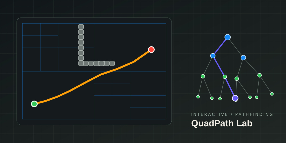
QuadPath Lab is a browser-based pathfinding workbench that joins spatial subdivision, graph search and interactive visualization into one pipeline: build a quadtree from a grid, derive an adjacency graph from its traversable leaves, then let A* or Dijkstra find a route through it.
What each concept is responsible for
A quadtree answers “how should the space be represented?” A regular grid treats every cell as a separate node. A quadtree begins with the entire map and recursively splits it into four. A uniform region becomes one large leaf; only a mixed region containing both free and blocked cells is subdivided again. Open space can therefore be summarized by a few large nodes while obstacle boundaries retain detail.
Dijkstra answers “how do we guarantee the shortest route?” Starting at the source, it always expands the node with the smallest accumulated cost. It makes no guess about the direction of the goal. With non-negative edge weights it finds a shortest path, although it usually explores more broadly.
A* answers “how can we search for that route with more direction?” It combines Dijkstra’s accumulated cost g(n) with a heuristic estimate h(n) to the goal and orders expansion by f(n) = g(n) + h(n). The Lab uses geometric distance as the heuristic, so the search tends to concentrate toward the destination.
Their relationship can be summarized as:
Grid map
  ↓ recursive subdivision
Quadtree leaves
  ↓ spatial adjacency and movement cost
Searchable graph
  ├─ Dijkstra: cost already travelled
  └─ A*: travelled cost + estimate to the goal
The quadtree is not a third pathfinding algorithm and it does not replace A* or Dijkstra. It reduces and organizes the search space; the two algorithms decide how to move through that space.
How the pieces are integrated
Whenever the map changes, the Lab rebuilds the quadtree and collects every traversable leaf. Two free leaves are connected when their regions share a boundary, and the edge weight comes from the geometric distance between their centers. The start and goal are mapped to the leaves that contain them, then both algorithms run on exactly the same graph.
That makes the comparison fair: spatial structure, endpoints and edge weights remain identical. Only the expansion strategy changes. Each run records visit order, final path, expanded-node count, path length and computation time.
Blue regions on the map show spatial nodes already expanded by the search; the orange polyline is the final route. The inspector on the right explains how map regions were recursively divided. The D3 force-directed window shows the parent-child hierarchy of the quadtree, not the adjacency graph used for pathfinding. Purple links mark the hierarchy path from the root to the selected node.
How to use the Lab
- Pick Offset Corridors, Connected Rooms or Open Field, or change the row and column counts yourself.
- Edit the map with obstacle, erase, start and goal tools. The quadtree is rebuilt immediately after every change.
- Choose A* or Dijkstra and press Run to start the search animation.
- Use playback, single-step and speed controls to inspect expansion order, then compare measured runs in the Results tab.
- In Inspect mode, click a map region to locate its tree node. Move deeper through the quadrant navigator to see how each level covers the original map.
- Open Topology for a movable window. Drag nodes, zoom the canvas, collapse subtrees or rebuild the layout while keeping the map visible behind it.
- Switch between Chinese and English or light and dark themes from the upper-right controls. All computation stays in the current browser; map data is never uploaded.
The point is not merely to watch an algorithm draw a line. It is to see how spatial representation changes the size of the search problem, and why two strategies explore the same graph in visibly different ways.